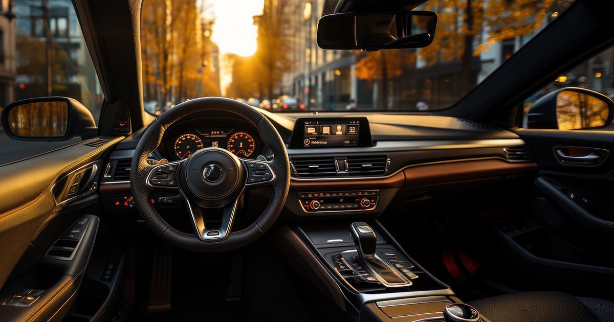
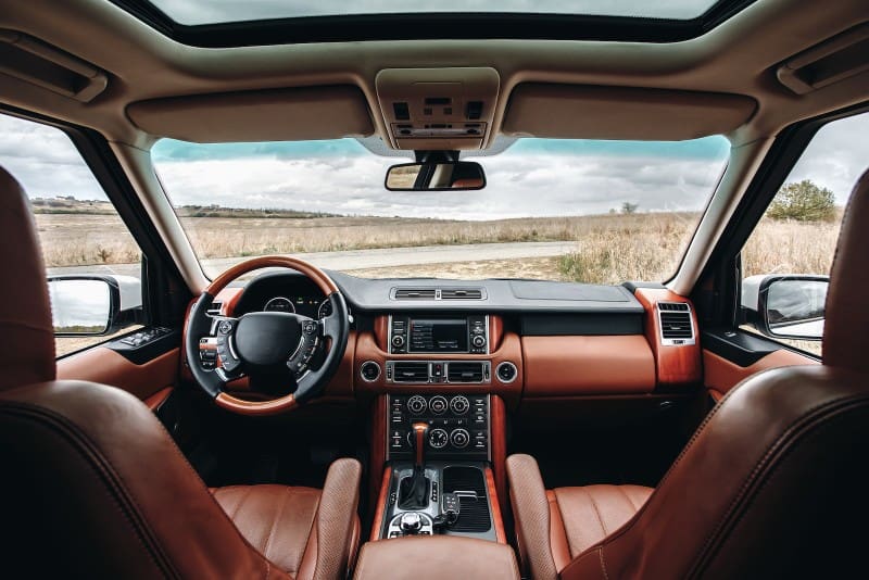
Clear Vibrations

Quakertown, PA's Mobile Enhancement Headquarters

550 California Road Suite 7
Quakertown, PA 18951
267-227-3875
  • Home
  • Services
    • Car Audio
    • Custom Installation
    • Driver Safety
    • Fleet Services
    • Remote Car Starters
  • About Us
    • Work for Clear Vibrations
  • Reviews
  • Location
  • Contact Us
  • Facebook
  • Instagram
  • Twitter
  • YouTube

Why Battery Voltage is Key to Your Car Audio Amp’s Performance

Battery Voltage

A short while ago, while testing an amplifier’s maximum power output, we observed how significantly the power increased with higher supply voltage. This observation made us realize that we’ve never thoroughly examined the relationship between a vehicle’s battery voltage and a car audio amplifier’s maximum power output. It’s time to address that.

Why Does Battery Voltage Matter to Amplifier Power Production?

Today, most car audio amplifiers use loosely or completely unregulated power supplies. As a result, the positive and negative voltages available to feed the output devices become a fixed multiple of the supply voltage. For instance, if the battery rests at 12.5 volts, an amp might generate 500 watts. However, if that voltage increases to 14.4 volts, the amp might produce 600 watts.

Maximum Supply Voltage Limits

To ensure product reliability, companies typically set a maximum voltage limit, which prevents the amp from producing excessive power. But why is this important? All car audio amplifiers convert some of the power they consume into heat. The heatsink and cooling system must dissipate a specific amount of heat energy to control the amp’s temperature. Notably, as the power level increases, the heat that needs to be expelled also rises because amplifier efficiency remains constant at maximum power.

For example, consider an amplifier that is 80% efficient and produces 500 watts of power; it converts 125 watts into heat. If provided with more supply voltage, the amp might produce 600 watts, requiring the heatsink to manage 150 watts of heat. This is likely manageable. Now, if the amp could produce 700 watts at 16 volts, it would have to manage 175 watts of heat—a significant increase from 125 watts. Unless the chassis is massive or there are numerous 0.3 watts, stepping from 14 to 15 volts increased the output by 56 watts.

Why does the power level increase more with each voltage jump? Power is proportional to the square of the voltage divided by the load resistance, according to the formula V^2 ÷ R. Thus, a slight increase in voltage results in a moderate power increase.

How Can You Maximize Voltage to Your Car Audio Amplifier?

Without resorting to unreliable aftermarket alternators or maintaining battery banks, the simplest way to ensure your amplifier receives all the power your battery and charging system produce is to have the technician working on the vehicle install a high-quality, all-copper power cable large enough for the amplifier’s current requirements.

In a car audio installation requiring about 15 feet of power wire, we suggest the following cable sizes: 10-AWG for loads up to 22 amps, 8-AWG for loads up to 35 amps, and 6-AWG (if you can still find it) for loads up to 56 amps. For loads up to 88 amps, a 4-AWG cable suffices. If you must pass 218 amps of current over 15 feet, a cooling fans, this difference means the amp won’t run as long before overheating.

Moreover, increased supply voltage presents another issue: the maximum voltage ratings on components. For example, most amplifiers include filtering capacitors on the power connections, which might be 16-volt, 1000 μF units. To accept more than 16 volts, the manufacturer might need to upgrade to 25-volt capacitors. These higher-voltage capacitors are larger and more expensive. Additionally, diodes and other protection circuitry components might need upgrades to handle higher operating voltages, further increasing costs with little performance gain under normal conditions.

Battery Voltage
High-quality car audio amplifiers will have capacitors on the power connections to reduce noise and store energy.

Testing Amplifier Maximum Power Output

We decided to test this further using a Rockford Fosgate Punch-Series P300X2 two-channel, full-range amplifier. Recently, we re-tested several amps with our new power supplies, and although this amp wasn’t on the schedule, we decided to test it anyway.

We set up the amp and connected it to a bank of 300-watt, low-inductance ceramic power resistors configured for a four-ohm load. Initially, we set the power supply to provide 16 volts to the amp, just under its maximum upper voltage limit. We then increased the signal to the amp until the output signal was within 1 to 1.05% THD+N. Afterward, we decreased the supply voltage and signal, measuring power output at 0.5-volt intervals until reaching the minimum power output of the power supplies. To comply with the ANSI/CTA-2006-D car audio amplifier power measurement standard, we measured power at 14.4 volts instead of 14.5 volts.

Battery Voltage

The difference in power output between 11.25 and 16 volts is substantial, as the chart shows. With an increase of 4.8 volts, the amp nearly doubled its power output. We simultaneously captured current draw measurements to calculate efficiency. This class-BD amplifier remained between 67% and 68% efficient throughout the entire range of measurements.

In our full Test Drive Review of the amplifier, our original maximum power rating was 360.1 watts at 14.15 volts. This time, we measured 398 watts at 14.4 volts. While you likely won’t hear the 38-watt difference, it’s worth noting that an amp rated to produce 300 watts made 400 watts. Rockford Fosgate fans already know they’re getting more than they paid for.

Plotting Amplifier Power vs. Battery Voltage

Let’s examine that chart as a graph.

Battery Voltage
Amplifier power output at 1% THD+N (+5, -0%) versus battery voltage.

Interestingly, while the relationship between the maximum power an amp can produce and the supply voltage appears linear, it’s not. The increase from roughly 12 to 13 volts yielded 48.3 more watts. The jump from 13 to 14 volts added 50-AWG power cable is necessary. For up to 289 amps, use a 2/0-AWG cable. Finally, if you have a massive amplifier or multiple smaller amps, 4/0-AWG cable over 15 feet is suitable for 422 amps. While these cables can undoubtedly pass more current, the voltage drop for these calculations is set not to exceed 0.35 volts over the entire length. Don’t forget to account for losses in the return path, which, if the cabling size and length are the same, would result in a 0.7-volt drop.

The Math on Power Output Versus Power Wire Size

To illustrate more clearly, for our 300-watt amplifier, losing 0.7 volts at the power terminals reduces the output by around 35 watts, roughly 10% of the rated power. If you think skimping on a power cable is a good idea, here’s the math to prove otherwise.

Consider this amp’s maximum theoretical power output with 15 feet of 10, 8, and 4-AWG cables for power and ground connections. Assuming the electrical system could maintain 14.4 volts at the battery, a 15-foot run of 10-AWG power and ground cable would reduce the voltage at the amp to 13.11 volts. With 8-AWG cables, the voltage would drop to 13.59 volts, while using 4-AWG cables reduces the drop to 14.08 volts. If you splurged on 0-AWG cable, the drop across the cable would result in the amp receiving 14.27 volts. You might have expected less drop across 30 feet of 0-AWG power wire, but that’s not the case.

If you’re curious why Rockford Fosgate overrates its amplifiers, it’s because most installations lack adequately large power and ground cables. If you waste a volt across the power wire, in the case of the Punch P300X2, the maximum power output drops by about 10%. You’ll still get all the power you paid for, but not as much as possible. Therefore, investing in larger power and ground cables is more cost-effective than buying the next-size car audio amplifier in a series.

Battery Voltage
Rockford Fosgate’s 1/0 AWG power wire is CTA-2015 and BC-5W2 compliant.
Battery Voltage
KICKER’s 1/0 power wire is 100% OFC and meets the full American Wire Gauge (AWG) size specification.
Battery Voltage
Audison Connection 1/0 power wire was one of the first super-flexible designs and is tinned for marine applications.

Don’t Starve Your Car Audio Amp for Voltage

Even after an average of three and a half decades in the mobile enhancement industry, none of our team members recall anyone publishing similar data. It may have happened, but we haven’t seen it. This data highlights the critical need for adequately sized power cables. If you’re considering upgrading your car audio system with high-power amplifiers, ensure the wiring is sufficient to maximize the power output from your chosen amp. Visit a local specialty mobile enhancement retailer today. Choose an amplifier that sounds great and is efficient, then ensure it is installed with the largest power and ground cables you can afford.

This article is written and produced by the team at www.BestCarAudio.com. Reproduction or use of any kind is prohibited without the express written permission of 1sixty8 media.

Filed Under: ARTICLES, Car Audio, RESOURCE LIBRARY

DSP Features You Might Not Have Known Existed

DSP Features

When 99% of car audio enthusiasts think about a digital signal processor (DSP), they associate it with equalizers, crossovers, and signal delays. In more advanced solutions, a consumer-grade car audio DSP might add the ability to include all-pass filters, an upmixer for a center channel and signal summing. However, at an engineering level, much more is available. Let’s look at a handful of DSP features that make audio systems at home, work, and on the road sound better.

What is a Digital Signal Processor?

Before we discuss some of the hidden features in digital signal processors, we should define them. A DSP is a microprocessor designed specifically to perform high-speed numerical calculations to process signals. Digital signal processors are used in video transmission, radio frequency systems, and audio systems. They are also used to interpret and manipulate sensor data in commercial, industrial, and research applications.

DSP Features
Many modern radar detectors use DSP to process the information from the radar antenna to improve range.
DSP Features
The cameras used for Lane Keep Assist and Adaptive Cruise Control use digital signal processing to interpret image data. Image: Ansys, Inc.

In short, a DSP can take a stream of digital data and manipulate or extract information from it extremely quickly. Our smartphones, smart speakers, digital cameras, drone quadcopters, smartwatches, and security cameras use this technology to provide the features, functionality, and performance you want.

Audio DSP Development

As a little peek behind the curtain, we want to introduce you to an audio DSP development suite called Analog Devices SigmaStudio. The technicians and engineers who develop car audio signal processors from scratch use this tool as part of the development process. It works like a flowchart. The designer can drag and drop elements into the project and then link them together. They would then write code in their interface to control the different elements in the DSP configuration. That’s a greatly simplified version of how it works, but you get the general idea. Writing a new DSP software package from scratch takes over ten thousand man-hours, making it a very expensive and time-consuming proposition. Testing that software also takes thousands of man-hours.

DSP Features
An example of a signal path in the Analog Devices SigmaStudio developer tool.

We are by no means experts in working with SigmaStudio, but its basic functionality is simple to follow. Looking at the image above, there is a stereo input on the left. One channel from that input feeds a volume control, which can be thought of as the gain. Then, the signal goes into a limiter, which we’ll discuss shortly. After that, there are three parametric equalization modules, followed by a filter module. Finally, we have an output. In theory, this setup would serve as a three-band equalizer and an adjustable crossover.

Hidden DSP Features – Audio Limiters

You might have noticed that the latest generation of factory-installed amplifiers in cars, trucks, and motorcycles are much less prone to damaging speakers. Is it that the speakers are now better? That’s part of why, but not the most significant factor. Many of these modern amplifiers have a limiter built in. A limiter will reduce the amplitude of a signal if it exceeds a certain threshold.

For example, if your installer turns up two bands of an equalizer with similar frequency centers, that might try adding 24 dB of signal at a specific frequency. A boost of 24 dB would take a 0.5-volt signal and increase it to 7.93 volts. That’s likely far more signal than an amplifier can accept.

We talked with our friends at Rockford Fosgate about the amplifier used on new Harley Davidson motorcycles. They incorporated several limiters into the design. As such, the amplifier won’t clip (overdrive) the outputs and add huge amounts of distortion, even if all the equalizer bands are boosted to their maximum levels. Similar features are integrated into some car audio amplifiers.

DSP Features
The new Rockford Fosgate Harley-Davidson amplifier can’t be driven to clipping, even with the volume cranked and the equalizer maxed out.

As a side note, anyone trying to measure power output on this amplifier with a device that looks for distortion will result in horribly inaccurate results. The output signal never reaches 1% THD, so units like the SMD DD-1 and D’Amore Engineering AMM-1 or AD-1 won’t accurately measure power. Audio analyzers like those from Audio Precision or QuantAsylum can measure output level and distortion. More importantly, these devices determine when the signal stops increasing in amplitude regardless of the harmonic and noise content.

Noise Gates

Many DSP solutions include a feature called a Noise Gate, which operates at the opposite end of the audio amplitude scale. A noise gate turns off the audio output circuitry when the signal drops below a preset level. This suppresses any background hiss or noise. As the music fades out, just when you might hear noise, the outputs turn off, leaving silence. Most modern recording studios use gating like this to help isolate a performer’s voice.

ARC Audio uses a similar approach to noise-gating with the LR1 remote level control in its signal processors. When the remote’s level is set to its lowest setting, the output devices are muted by a digital signal from the microprocessor.

DSP Features
ARC Audio’s DSPs have a programmable remote level control with an output mute option.

Bass Processing

If you’ve been around the block for a while, you might remember the Waves MaxxBass processor. This processing algorithm analyzes harmonic content in an audio stream and then filters out the low-frequency information. Yes, that’s right—it removes bass information. It then modulates the upper bass and lower midrange frequencies to make it sound like the deep bass is still there. It’s a very cool way to produce the perception of deep bass from a small speaker with limited excursion capabilities. Smartphones and smart speakers—we’re looking at you!

DSP Features
Super Bass and Subharmonic generators are common features in the SigmaStudio.

If we can remove bass information, then could we not add it? If you’ve ever experienced the AudioControl Epicenter or Wavtech bassRESTOR, you know what we’re discussing. Imagine a system that can analyze the harmonic content of an audio stream and then add audio information that’s an octave or two lower. It would be like having a super-grand piano capable of playing a fundamental of 13.75 or even 6.875 hertz. Your subwoofers might not like it, but it would be fun to try! Subharmonic generators are easily added functions already built into the SigmaStudio.

Stereo Width Expansion

By now, you’ve realized that signal processors are capable of much more than just equalization and filtering. Way back in the day, many portable speakers—called boom boxes or ghetto blasters—had a switch that made the sound coming from them seem much wider. The SigmaStudio includes a stereo expander control as well.

Some research shows that Philips Semiconductors used to offer an IC called a Spatial, Stereo, and pseudo-stereo sound circuit. This was introduced in 1985, which coincides with our memory of these functions.

DSP Features
Portable speakers in the 80s and 90s had a stereo expander function that was often based on the TDA3810 IC.

More Features Require More Space

The goal of this article is to provide some insight into how digital signal processors are used in different audio systems. Some devices you might think are simple are, in fact, quite complex in terms of audio processing. One that caught us off-guard is a smart speaker, of which the Apple HomePod is a perfect example.

Anytime you have microphones and speakers, you can measure the sound in the time and frequency domains. In the case of the HomePod, the unit can use its microphone array to evaluate the acoustics of the environment it’s used in. For example, if the speaker is 12 inches from a wall, frequencies around 283 and 849 hertz are likely to be attenuated.

Sound Reflections Can Cause Cancellations

Sound emanates from all speakers in a spherical pattern below the frequency where it starts to be directional. The audio information that bounces off the wall behind the speaker will eventually mix with the sound coming directly to the listening position. In our example, we have a total distance of 24 inches added to the signal path—the distance from the speaker to the wall, then back to the speaker. Where the audio wavelengths match, but are inverted, the amplitude (volume) decreases around those frequencies.

Now, back to the HomePod and its signal processing. The system will have a benchmark for the time it takes for the sound to leave its speakers, arrive at its microphone, and then be processed. Let’s call this two milliseconds, to keep the math simple. If we have the HomePod in the middle of a table, it might be the aforementioned 12 inches from the wall. It takes sound 0.0008886 milliseconds to travel 12 inches. As such, it would take 1.777 milliseconds for the sound from the speakers to bounce off the wall and return to the microphone. Let’s add that processing time, and the DSP might measure a delay of 3.777 milliseconds. The math, calibrated in controlled testing conditions, knows there will be a dip in frequency response at 283 and 849 hertz. It can then apply equalization to those frequencies to produce a much smoother overall response for the listener.

Automatic Equalization

The system will also be able to measure the frequency response of the sound it hears. If it detects a constant increase in bass frequencies due to room resonance, it could theoretically adjust for this. We’ve heard many times that HomePods sound mediocre for the first few minutes they play. Then, they mute the audio for a second, load new equalization parameters, and continue playing. Everyone who’s heard them says they sound exponentially better after they recalibrate.

DSP Features
The Apple HomePod uses DSP-based measurements to self-calibrate itself for your chosen listening environment. Image: Apple Inc.

Many car audio digital signal processors have have the ability to make measurements, or work with external hardware to automate the process of setting signal delays and equalization. This is achievable thanks to the processing modules available for the DSP chips. We will note, it takes a LOT more code to make these work well. Add another ten thousand man-hours to that software development time.

Vehicle Presets

A simple DSP feature is the ability to load an entirely new calibration quickly. This is the same as we described above with the Apple HomePod. For example, if you drive a newer Ford Mustang convertible, you might notice that the audio pauses for a moment as you are raising or lowering the convertible top. This is the system loading a new audio system calibration. Your music should sound similar, at least in the midbass, midrange and high-frequency ranges. However, the settings used to achieve what you hear will be very different with the roof up or down.

DSP Features
The DSP built into the amplifier in late-model Ford Mustangs has two different audio calibrations—one for when the roof is up and another for when it’s down.

Real-Time Noise Cancellation

The last feature we’ll talk about is active noise cancellation. Many new cars and trucks come with an array of microphones integrated into the vehicle interior. The signals from these microphones are sent to a DSP for analysis. The DSP works out the frequency response of the sound from the microphones, then sends a signal with the opposite polarity to the audio system amplifier. When this new signal mixes with the road, exhaust, and wind noise in the car, it cancels. Again, the system is much more complex as timing is crucial to making this work. The result is a vehicle that’s quieter to drive, and that doesn’t incur weight penalties from massive amounts of sound deadening. Adding weight reduces fuel economy.

DSP Features
Companies like Silentium provide noise-canceling solutions to reduce sound levels with minimal weight penalties to automakers.

This same noise-canceling technology is used in headphones and earbuds.

DSP Features Improve Audio and Listening Experiences

We’ll step back to our discussion about car audio DSP features. Not all processors have all the technologies we’ve mentioned. Some solutions might use a chip that costs $5, while others might be $30. Every function added to a DSP increases the amount of memory required. As such, you might find that some inexpensive solutions have limited equalizer bands, whereas others have more than you might ever use. Further, you can’t just call a car audio company and say, “I know the Analog Devices chip can do this. Can you add this feature?” Having been on the other end of that, I guarantee it won’t happen quickly, if ever. It takes exponentially more time to develop and test the software than you can imagine. Even small changes require extensive lab and field testing. However, the lack of a feature is often attributable to parts costs and the coinciding lack of memory, or the fact that the company doesn’t develop their DSP in-house.

With that said, if your DSP has an upmixer for a center channel, bass restoration, automatic equalization, an RTA display, stereo width expansion or a whole slew of other features, you can thank the impressive processing power of modern digital signal processors.

Upgrade Your Car Audio System with a DSP, Today!

Digital signal processors are everywhere these days, often in devices we think are much simpler than they actually are. We hope learning about how digital signal processors work in general terms has been enlightening. If you are looking for a way to improve the performance of your car audio system, drop by a local specialist mobile enhancement retailer and ask them about adding a DSP to your audio system. Assuming the system is designed, integrated, configured and calibrated properly, the DSP upgrade will be stunning!

This article is written and produced by the team at www.BestCarAudio.com. Reproduction or use of any kind is prohibited without the express written permission of 1sixty8 media.

Filed Under: ARTICLES, Car Audio, RESOURCE LIBRARY

How Audio Signals Sum Around Crossover Points

Crossover point

Crossovers are an essential part of designing any audio system. From the passive designs used with a bookshelf or floor-standing speaker to three- and four-way electronic designs employed in car audio systems, ensuring signals combine correctly is crucial for delivering great sound. Crossovers can have different frequencies, slopes, and alignments. Understanding how audio signals from two speakers combine after being filtered is essential for creating exceptional audio systems. Let’s analyze the output of different crossover point alignments and slopes.

What is a Crossover?

In the simplest terms, a crossover is a circuit that allows your installer to divide audio frequencies into different parts. We’ll discuss two types of crossovers today—high-pass and low-pass. A high-pass filter allows audio signals above the crossover point to pass through, while a low-pass filter permits audio information that’s lower in frequency to go through.

In a simple two-way speaker design, like those found in a component set or small bookshelf speakers, the designer will include a high-pass filter for the tweeter and a low-pass filter for the midrange driver.

The primary purpose of the high-pass filter in this application is to limit the amount of midrange and low-frequency energy going to the tweeter. Tweeters have almost no cone or diaphragm excursion capability. That doesn’t mean they don’t move back and forth; they do. However, they only move by a tiny fraction of an inch. For example, if you send audio information below 300 hertz to a tweeter, it will physically bottom out and likely be destroyed.

Small Speaker Protection

Secondly, and more specifically for tweeters, audio information contains more energy at lower frequencies. A tweeter might have a 75 to 100-watt power rating; however, this rating would be determined with something like a 5 kHz filter in place. As such, the driver will likely only ever see a small fraction of the total power.

The image below shows the spectral response of pink noise. We often use pink noise in audio system configuration and calibration as it represents how we hear music. To put it another way, this sloped red line sounds like there is an equal amount of energy in the bass, midbass, midrange, and high-frequency regions.

Crossover point
A graph of pink noise in red and the signal to a tweeter after a 5 kHz 12 dB/octave filter has been applied in green.

The green line is the same pink noise track, but we’ve applied a 5 kHz 12 dB/octave high-pass filter to the signal. You can see that the peak energy level around 6.5 kHz is at -57 dB. The peak of the unfiltered pink noise is at -30 dB. If the pink noise were at 100 watts, then the tweeter would only see 0.2 watts. This is the process used to rate the power handling of tweeters. Yes, a 100-watt tweeter likely can’t handle more than 0.5 to 1 watt of power.

Crossover Characteristics – Frequency

The number one criterion in setting a crossover is selecting a crossover frequency. This frequency is where the output of the crossover is at the same level, whether configured as a high-pass or low-pass filter. For some types of crossovers, this point might be at -3 dB from the unfiltered level, while others might be at -6 dB.

Crossover point
High-pass (white) and low-pass (gray) crossovers set to 500 Hz.

The image above shows the predicted frequency responses of two crossovers. The white trace is a high-pass crossover set to 500 Hz, while the gray line is a low-pass crossover set to 500 Hz. As you can see, the crossovers intersect at precisely 500 Hz. Furthermore, the amplitude, or output level, is at -3 dB at this frequency.

Crossover Characteristics – Slope

As you can see in the image above, some audio on the other side of the crossover passes through the filter. The rate at which the signal is attenuated is called the slope. We describe slopes in decibels per octave. In the example above, for every octave we move away from the crossover point, the output is 12 dB lower. This is called a -12 dB/octave crossover.

For most car audio applications, especially when considering the crossovers in a radio, amplifier, or digital signal processor, we usually use -12 dB/octave or -24 dB/octave. There are other options, though. A -6 dB/octave filter mimics the response of adding a capacitor or inductor in series with a speaker. Slopes in source units and digital signal processors rarely exceed -48 dB/octave. That said, -24 dB/octave provides a good balance of speaker protection without too much effect on phase. We’ll explain the phase shortly.

Crossover point
Examples of -6 dB (white), -12 dB (gray), -18 dB (green), and -24 dB/octave (violet) 500 Hz high-pass filter slopes.

Crossover Characteristics – Alignments

The math or physical characteristics of how a crossover works can vary dramatically from one implementation to another. You might have heard of Butterworth, Linkwitz-Riley, Bessel, and Chebyshev crossover alignments. These names describe the attenuation rate, frequency response, phase response, and behavior at the crossover point.

Crossover point
A comparison of -12 dB/octave Butterworth (white), Linkwitz-Riley (gray), Bessel (green), and Chebyshev (violet) crossover alignments.

Each type of filter has its benefits and drawbacks. To be clear, a filter’s frequency response describes how two signals sum around the crossover point. This is the crux of this article. We use crossovers to filter and protect smaller speakers but not reduce audio quality.

We could write an article on each of the different crossover alignments. For our discussion in this article, we will focus on Butterworth and Linkwitz-Riley, which are commonly found in digital signal processors and many car audio amplifiers.

Don’t Get Phased

Before we look at how different crossovers sum back together, we need to talk about phase. Phase is the change in time of an AC waveform relative to a reference. You can’t have phase without being able to compare it to something. So, two waveforms might be in phase if each cycle starts and stops at the same point in time. Two waveforms would be described as out of phase if one was moving upwards when the other was moving downward. Here are a few simulated waveforms on our MegaScope to help you visualize this concept.

Crossover point
The violet and green audio waveforms cross the 0-line at the same point. They are in phase.

In the above example, the violet and green waveforms have different amplitudes but cross the 0-line at the same point. This indicates they are in phase and have the same frequency. The blue line represents the sum of the waveforms.

Crossover point
The violet and green waveforms cross the 0-line at the same point but travel in opposite directions. These waveforms would be described as having reversed polarity.

In this second example, two waveforms start at the same point in time and cross the 0-line at the same point. This means the waveforms have the same frequency. However, when one waveform moves upward, the other moves down. We describe this as having reversed polarity. This is NOT the same as being “out of phase.” When we add the amplitudes, we get 0, as shown by the blue line.

Crossover point
Two waveforms that start at different points in time.

This graph shows that the violet waveform starts a 1/4-cycle after the green. These waveforms are described as being out of phase. They have the same frequency and amplitude, but they don’t cross the 0-line at the same time. The critical consideration here is the starting time.

Phase is a complex topic that can be difficult to grasp. Improper terminology adds to the confusion.

One last tidbit of complexity before we move on: We describe the point in a waveform using degrees. One complete cycle is 360 degrees. This would be where the waveform crosses the 0-line, moving upwards to where that repeats. If a waveform starts half a cycle late, we describe it as being 180 degrees out of phase. Understanding that this delayed start is NOT the same as having opposite or reversed polarity is crucial.

Phase and Crossover Alignments – First Order

Now that we have a foundational understanding of the factors that define crossovers and some knowledge of phase, we can discuss phase specifically related to crossover slopes. All crossovers can be described using the term order. A first-order crossover has a slope of -6 dB/octave. At the crossover frequency, the signal phase will have shifted by 90 degrees.

Crossover point
First-order high-pass filter amplitude (white) and phase (dotted white) response. First-order low-pass filter amplitude (gray) and phase (dotted gray) response.

The image above shows a 45-degree phase shift at the 500 Hz crossover point for a first-order high-pass filter. This means the start and stop points of a 500 Hz waveform are delayed by 1/8 of a cycle. A low-pass filter has a -45-degree phase shift, meaning the waveform would be 1/8 of a cycle ahead or earlier than if there were no filter. This 90-degree difference in phase between the two signals makes it very difficult to add the output of two first-order filters back together.

Crossover point
Waveforms with a 90-degree phase shift as seen on an oscilloscope.

Phase and Crossover Alignments – Second Order

If we looked at two 16-volt peak-to-peak 500 Hz waveforms on an oscilloscope, we’d see they sum to only 22.6, not 32 volts. This would present a dip in the frequency response at the crossover point.

Crossover point
Second-order high-pass filter amplitude (white) and phase (dotted white) response. Second-order low-pass filter amplitude (gray) and phase (dotted gray) response.

We now have second-order filters with the crossover slopes increased to -12 dB/octave. The 500 Hz crossover point phase is now 90 degrees for the high-pass and -90 degrees for the low-pass filter. If we sum the output of these filters together, the waveforms will cancel each other out because their phase relationships are 180 degrees apart.

Crossover point
Waveforms with a 180-degree phase shift as seen on an oscilloscope.

Phase and Crossover Alignments – Third Order

Crossover point
Third-order high-pass filter amplitude (white) and phase (dotted white) response. Third-order low-pass filter amplitude (gray) and phase (dotted gray) response.

Our third-order filters shift 135 degrees for the high-pass and -135 degrees for the low-pass. Once again, summing with third-order filters is difficult due to the 270-degree phase mismatch at the crossover frequency.

Crossover point
Third-order high-pass filter amplitude (white) and phase (dotted white) response. Third-order low-pass filter amplitude (gray) and phase (dotted gray) response.

With a fourth-order filter, the high-pass filter has a 180-degree phase shift at the crossover frequency of 500 Hz, while the low-pass filter has a phase shift of -180 degrees at the same frequency. The difference is 360 degrees, which results in perfect summing at the crossover point.

Crossover point
Third-order high-pass filter amplitude (white) and phase (dotted white) response. Third-order low-pass filter amplitude (gray) and phase (dotted gray) response.

Signal Summing and Voltage

If you’re considering how signals sum and how crossovers affect phase response, those second-order filters should raise a red flag. We created several pink noise tracks in Adobe Audition and then applied high-pass and low-pass filters to them. Finally, we combined them back into a single track. The image below shows the resulting frequency response.

Crossover point
Pink noise filtered with a second-order low-pass filter – yellow. Pink noise with a second-order high-pass filter – green. Filtered signals summed back together – teal.

As predicted, we have a massive notch at the crossover point. There’s an easy fix for this, though. All we have to do is invert the polarity of one of the signals. Here are the same summing process results but with the high-pass filter signal inverted.

Crossover point
Pink noise filtered with a second-order low-pass filter – yellow. Pink noise with a second-order high-pass filter – green. Filtered signals summed back together – blue.

We don’t have a dip, but we have a 3 dB bump in output around the crossover point. Why is this? As mentioned, second-order Butterworth filters are down -3 dB at the crossover point. If two speakers are playing the same information at the same frequency, that increases output by 6 dB. Thus, -3 dB plus -3 dB is +3 dB. We need the output to be lower at the crossover point.

There may be a theoretical way to underlap the crossover to get the signal to sum flat, but that’s not a recommended or reliable configuration for an audio system and will likely result in unwanted phase issues.

Linkwitz-Riley Crossovers to the Rescue

It might not be a huge surprise, given that we’ve already shown the characteristics of the commonly available crossover alignments. However, Linkwitz-Riley crossovers are at -6 dB at their crossover point, sometimes called the knee frequency. Let’s rerun our simulation in Adobe Audition to see if the math checks out.

Crossover point
Pink noise filtered with a second-order low-pass filter – red. Pink noise with a second-order high-pass filter – orange. Filtered signals summed back together – violet.

As you can see, the signals are summed together to produce a smooth, flat response. However, we still had to invert the signal polarity of one of the waveforms, as the slopes remained at -12 dB.

Understanding Electronic Crossovers

As you can see, crossovers are much more complicated than most enthusiasts think. Using a calibrated real-time audio analyzer to ensure the frequency response around the crossover point of all the speakers in your vehicle is crucial for ensuring your system sounds its best. You might have a null at the crossover point with a subwoofer or a midbass to midrange driver. Equally unsatisfactory would be a bump in frequency response at a crossover point. Visit a local specialty mobile enhancement retailer today to start the process of improving the performance of your car audio system.

This article is written and produced by the team at www.BestCarAudio.com. Reproduction or use of any kind is prohibited without the express written permission of 1sixty8 media.

Filed Under: ARTICLES, Car Audio, RESOURCE LIBRARY

Unlocking the Secrets of Human Hearing: Understanding Weighting Curves in Audio

Weighting Curve

Though it might surprise you, human hearing is significantly more sensitive to some frequencies than others. You can think of this phenomenon as our built-in frequency response. However, unlike a speaker or amplifier, variations are not something we want to compensate for in an audio system—at least, not directly. Let’s discuss how human hearing works with respect to different frequencies and why we need to compensate for this when making sound or product specification measurements. All of this will tie together perfectly with an explanation of weighting curves.

Human Hearing and Frequency Response

Did you know that human hearing is most sensitive around 3.5 kHz? This is due to the dimensions of the ear canal, which typically resonate between 2 and 5 kHz. Even a faint sound at 3.5 kHz is easy to detect. A sound might need to be 10 dB louder at 350 hertz to be perceived as having the same loudness.

In 1933, Harvey Fletcher and Wilden Munsen performed a set of measurements to quantify human hearing concerning frequency and intensity perception. Their paper, “Loudness, Its Definition, Measurement and Calculation,” included what became known as the Fletcher-Munson curves.

Weighting Curve
The first attempt at quantifying loudness and human sensitivity resulted in the Fletcher-Munson curves.

The lines on the chart are separated into amplitude levels called Phons. The Phon is the unit of measure used to describe sounds perceived as equal in intensity. As such, they follow the equal loudness level contours proposed by Fletcher-Munson and subsequent iterations.

It shouldn’t be surprising that the test equipment used to generate test tones wasn’t as precise in 1933 as it is today. Similar testing in 1937 by Churcher and King and again in 1956 by Robinson and Dadson produced significantly different results.

Introducing the Equal Loudness Level Curves

The International Organization for Standardization (ISO) took over the creation of reference loudness curves in 2003. A study by Tohoku University, Japan, and the Research Institute of Electrical Communication showed errors as large as 15 dB from the original data. These new tests became the ISO 226:2003 Standard. Don’t think it’s over yet. These have since been revised again to the ISO 226:2023 Standard.

Weighitng Curve
The Equal Loudness Level Contour curves presented in the ISO 226:2023 standard are the reference for evaluating loudness.

Of course, the above curves are averaged across a wide selection of people of different shapes and sizes. Everyone’s hearing will be slightly different in the areas where it is most sensitive. However, this data provides an excellent overview.

If anyone references the Fletcher-Munson curves, they are at least four generations behind in their data. When discussing the perception of sound levels versus frequency, the proper reference is the ISO 226:2023 Equal Loudness Level Curves.

Interpreting Equal Loudness Level Curves

If you look at the 1 kHz point on each trace, you’ll see that this point coincides with the reference SPL value. So, a sound at 70 dB at 1 kHz is perceived as being at 70 Phons. However, it takes about 74 dB of energy at 1.5 kHz to seem as loud. Further, it takes only 67 dB of energy at 3 kHz to seem as loud.

What matters here are the extreme ends of each trace. We can make some generalized assumptions about human hearing based on the reduced sensitivity in these regions. Staying with the 70 dB trace, we would need to hear a sound that’s 83 dB at 10 kHz to be perceived as being as loud as 70 dB at 1 kHz. Further, a sound at 93 dB at 63 hertz is also perceived to be as loud as 70 dB at 1 kHz.

Though we haven’t consulted with an audiologist (yet), the issue is less about attenuation at opposite ends of the audio spectrum and more about an increase in sensitivity in the middle. As mentioned, the ear canal resonates around 2 to 5 kHz. Furthermore, the outer ear, called the pinna, also amplifies sounds in this frequency range.

The middle ear bones, the ossicles, are more efficient at transmitting mid-frequency sounds. An effective impedance mismatch between the air and the fluid in the cochlea further accentuates this frequency range.

There are additional mid-frequency sensitivities in the cochlea due to where different frequencies peak.

Audio System Equalization

We’ve seen many amateurs try to equalize their audio systems, more often in a home environment than in a vehicle, to compensate for the shape of these curves. That’s not the purpose of the information. Our perception of hearing is static. In short, we hear what we hear. We accept that the sound of a trumpet or saxophone is what it is. We don’t want to change that presentation to compensate for being more sensitive in one range versus another.

There is an exception to this statement. Regarding headphones and earbuds, flat response doesn’t sound accurate. This is because we’ve eliminated some of the frequency filtering caused by the pinna. As such, a modified response curve sounds best. The team at Harman International has devoted significant time and expense to creating a target curve for headphones based on similar experimentation that created the Equal Loudness Level Curves.

Weighting Curve
Harman has invested heavily in research to evaluate what response listeners prefer to create a target headphone curve.

Analyzing Headphone Target Frequency Response

There are two critical pieces of information to extract from the above response graph. First, we can see the boost around 3.5 kHz that coincides with the boost the pinna of our ears adds. Without this, headphones would sound dull and flat. Second, there is a boost in low-frequency information. Part of this will be due to the Equal Loudness Level Curves, and part will be listener preference. We all know that many people prefer bass information boosted in their listening systems. The Harman headphone curve combines the science and mechanics of human hearing with extensive listener preference. They even have details on the percentage of people who prefer more bass and less bass.

Harman uses very specific test equipment to measure headphones. Specifically, a head and torso simulator accurately and repeatably simulates how humans perceive sound.

Weighting Curve
The Bruel and Kjaer HATS 5128 high-frequency head and torso simulator is the benchmark for accurate sound measurements.

It’s worth noting that Harman has revised its target curve from the one shown above. Unlike this first iteration, they are not releasing this new curve to the public for endless debate and whining (insert sarcastic wink here!). They will use it to fine-tune the performance of their AKG, Mark Levinson, Harman Kardon, and JBL consumer and professional products.

Speaker Evaluations in Free Field Conditions

If we measure the frequency response of a conventional loudspeaker using a sine sweep or pink noise, we should end up with a fairly flat line, assuming the speaker can play from 20 Hz to 20 kHz with good accuracy. Most floor-standing home speakers roll off below 30 Hz. It would be best to have a dedicated subwoofer to fill in that bottom octave.

The chart below represents a nearly perfect speaker’s ideal frequency response. Do you think if we suck up to KEF enough that they will loan us a set of Blade 2 Meta to use as our reference review speakers? Here’s hoping!

Weighting Curve
Above 250 hertz, the KEF Blade 2 Meta’s frequency response is ruler flat. Image: Stereophile magazine.

As noted in Stereophile Magazine’s review of the Blade 2 Meta, the boost in the bass is primarily due to the close-micing technique used for measurements.

A-Weighting Curves in Measurements

Let’s get to the nitty-gritty of this article. Look at the Equal Loudness Level Curve chart above and analyze the 40-phon trace. Information similar to this was used to create what’s known as the A-weighting curve. This curve is intended to be applied to a sound pressure measurement so that the energy in the measurement correlates to how we hear. It was actually the Fletcher-Munson 40-phon curve that was used to create the A-weighting curve. Thankfully, the ISO 233-2032 40-phon curve is quite similar.

Weighting Curve
The chart above shows the response of the A-weighting curve.

To show you the same data in a format you might be more familiar with, we dug out the Sony XM-4ES amplifier we reviewed a few years back. We performed a frequency response test with all the settings flat and again with the A-weighting filter activated in the QuantAsylum software.

Weighting Curve
Frequency Response of the Sony XM-4ES with no weighting filter applied.


Weighting Curve
Frequency Response of the Sony XM-4ES with an A-weighting filter applied.

Where We Use Weighted Measurements

The ANSI/CTA-2006-D standard for measuring car audio amplifiers calls for applying the A-weighting curve to the measurement after the reference level is set. Up to this point, we’ve shown the measurements as unweighted. The result is slightly lower values, indicating the presence of more noise. As we move to further comply with ANSI/CTA-2006-D, we’ll start using the A-weighting curve to evaluate the signal-to-noise ratio of the source units’ amplifiers and signal processors we test.

Weighting Curve
An example of a signal-to-noise ratio measurement made without any weighting.

We can see that the Signal-to-Noise Ratio measurement of this Sony XM-4ES amplifier is specified as being 71.23 dB.

Now, if we turn on the A-weighting filter and apply it to the measurement, the low- and high-frequency information is attenuated, which reduces its effect on the measurement.

Weighting Curve
An example of a signal-to-noise ratio measurement made with an A-weighted measurement.

The QuantAsylum software has revised the SNR measurement to -76.11 dBA. The addition of the letter A after dB indicates the use of A-weighting. Given the published measurements on the CTA TECH website, which show -76.5 dBA for the XM-8ES and -80.8 dBA for the XM-6ES, we are comfortable saying our data aligns with those numbers.

So, the next time you see a signal-to-noise ratio measurement with the amplitude specified in dBA, you will understand how and why that rating system is used. Finally, a higher SNR number means that the noise is further below the test signal. A level of -75 dBA is about the minimum you’ll want to consider for an amplifier in a car audio system that will drive midrange and high-frequency speakers.

This article is written and produced by the team at www.BestCarAudio.com. Reproduction or use of any kind is prohibited without the express written permission of 1sixty8 media.

Filed Under: ARTICLES, Car Audio, RESOURCE LIBRARY

CarPlay Sound Quality Face-Off: Wired vs. Wireless—Which Is Better?

Wired CarPlay Sound Quality

A reader requested that we compare the sound quality performance of wired and wireless Apple CarPlay. This is a great idea, as very little information is provided about the communication standards used to send audio signals wirelessly to a source unit. So, let’s look at distortion characteristics and frequency response to see if there is a performance difference.

The Test Configuration

While our lab has an impressive selection of car radios, we didn’t have one that supports both wireless and wired CarPlay. We contacted our friend Lee Mattason at Burlington Radioactive for help. He graciously lent us a Kenwood eXcelon DMX908S to make some measurements. If you live in the Golden Horseshoe region of Southern Ontario and are looking for a car, boat, or motorcycle audio upgrade, Lee and his team are a great choice.

We are going to perform two different tests using four connectivity criteria. We will analyze sound quality by playing a 0 dB 1 kHz test tone and then analyzing it for harmonic content. The second test will evaluate frequency response by analyzing a white noise track. In both cases, the test tracks have 44.1 kHz sampling rates and are stored with 16 bits of depth. To ensure Apple didn’t alter the file while uploading it to the phone, we used the Onkyo HF Player and copied the tracks as files to a specific folder on the iPhone. The device is an Apple iPhone 14 Pro running iOS 18 Beta 2. Please don’t ask why the owner tries beta software on this phone—it’s a terrible idea.

The four communication methods we’ll use are playing the files from a USB memory stick, over a Bluetooth connection, through Apple CarPlay with the phone connected to the radio with a Lightning cable, and finally, using Wireless Apple CarPlay.

USB Media File Playback

The first test is to play the 1 kHz test tone track directly from the USB stick. We’ll note that with all the audio settings turned off and the source-specific levels flat, we saw an output of 4.539 volts on the front RCA output. The signal had a THD+N measurement of 0.01086%, which is excellent for a consumer-grade source unit. The signal-to-noise ratio (SNR) came in at -85.39 dB, unweighted.

Wired CarPlay Sound Quality
The 1 kHz test track played from a USB memory stick.

Next, we have a 10-minute white noise track. We cranked up the averaging on the QA403 audio analyzer to produce as flat of a measurement as possible. The goal in interpreting the data below is to average the frequency response in your mind. We’d call this flat from below 20 Hz to 22 kHz on the top end. This is precisely what you’d expect from this measurement.

CarPlay Sonud Quality
White noise played from a USB stick and averaged for more than a minute.

These measurements will serve as a solid baseline to compare with other playback media.

Bluetooth File Playback

We all know that the iPhone isn’t the go-to for Bluetooth sound quality. The use of Bluetooth 5.3, specifically with the SBC codec, really limits performance compared to an Android-based device that offers something spicier, like LDAC or aptX HD. For now, this is the test, and we’ll hunt down an Android phone and give that a go in a future article.

Let’s start with the distortion measurement. In a word, we can sum this up as being subpar. We can see all sorts of artifacts and harmonics starting at -46 dBV. This gives us a THD+N specification of only 0.14655% and a signal-to-noise ratio of 56.83 dB.

Apple CarPlay Sound Quality
Spectral analysis of our 1 kHz test tone streamed over Bluetooth.

In terms of frequency response, the curve remains nice and flat, so overall, music would sound generally the same. The increase in distortion shown above hampers clarity and could add some emphasis. However, the raw amplitude measurements are similar. Looking closely, you can see that the high-frequency information rolls off at about 17.5 or 18 kHz. None of us can hear anything above 18 kHz, so that’s not a massive concern.

Apple CarPlay Sound Quality
White noise played over the iPhone’s Bluetooth connection.

Wireless Apple CarPlay

We deleted the Bluetooth pairing from the radio and phone and reestablished it to turn on Apple CarPlay. We were cautious in all the tests to ensure the communication used our desired method.

Starting with the 1 kHz tone, we can see that the Wireless Apple CarPlay connection uses Bluetooth to transmit audio to the source unit. The distortion numbers are slightly worse at 0.15072%, and the SNR is -56.62 dB unweighted. If you are fanatical about sound quality, this isn’t the best way to get music from your phone to your radio.

Apple CarPlay Sound Quality
Spectral analysis of our 1 kHz test tone streamed using Wireless Apple CarPlay.

Using Wireless CarPlay, the high-frequency information is attenuated a little more than when using a Bluetooth-only connection. We’d say the audio information stopped around 17-17.5 kHz. Once again, this won’t be audible to most people. However, it’s repeatably measurable and very real.

Apple CarPlay Sound Quality
White noise played using the Wireless Apple CarPlay connection.

Wired Apple CarPlay

Last but certainly not least, it’s time to see how the combination works with a wired connection between the iPhone and the Kenwood radio. We deleted the phone pairing from both devices and plugged the phone into the micro-USB port on the back of the chassis.

For the 1 kHz tone, we saw a THD+N measurement of 0.01042%, which is the best of this test session. The signal-to-noise ratio came in at -85.21 dB. Both numbers are inconsequentially different from the original USB test. Nobody would be able to hear the difference in clarity or background level between Wired Apple CarPlay and playing an audio file from a USB memory stick.

Apple CarPlay Sound Quality
Spectral analysis of our 1 kHz test tone streamed using a wired Apple CarPlay connection.

We also have the spectral analysis of the white noise when played over a wired CarPlay connection. It looks nearly identical to the wireless connection. Again, even a variation from 17.5 to 20+ kHz isn’t audible to humans. Your pet cat, Fluffy or Wayne, or the neighborhood bat might disagree.

Apple CarPlay Sound Quality
White noise played using the Wired Apple CarPlay connection.

Conclusions on Apple CarPlay Audio Playback Quality

Based on this specific test, we’d say there is an audible difference in clarity between wired and wireless connections. Whether you are using Bluetooth or Wireless Apple CarPlay, you leave a significant amount of audio clarity performance on the table compared to Wired CarPlay or a USB memory stick. However, this is a single test with one specific radio and phone combination. It’s possible that an Android phone would fare much better wirelessly. We’ll make that test happen soon!

It’s also worth noting that the clarity difference might be easy to hear when sitting in the car with the engine off but much harder when you’re driving down the Interstate. Background noise masks a lot of distortion. However, we’d use a wired connection every chance we could.

If you are shopping for a new radio with Apple CarPlay and Android Auto, drop by a local specialty mobile enhancement retailer and ask what they have that will fit your vehicle. Be sure to bring your phone to connect it and ensure the radio works exactly how you want.

This article is written and produced by the team at www.BestCarAudio.com. Reproduction or use of any kind is prohibited without the express written permission of 1sixty8 media.

Filed Under: ARTICLES, Car Audio, RESOURCE LIBRARY

  • 1
  • 2
  • 3
  • …
  • 81
  • Next Page »

Recent Articles

A lot of car audio equipment set up in the back of an SUV

Why Battery Voltage is Key to Your Car Audio Amp’s Performance

November 23, 2025 

A short while ago, while testing an amplifier's maximum power output, we observed how significantly the power increased with higher supply voltage. This observation made us realize … [Read More...]

DSP Features You Might Not Have Known Existed

DSP Features You Might Not Have Known Existed

November 16, 2025 

When 99% of car audio enthusiasts think about a digital signal processor (DSP), they associate it with equalizers, crossovers, and signal delays. In more advanced solutions, a … [Read More...]

How-Audio-Signals-Sum-Around-Crossover-Points-Lead-in

How Audio Signals Sum Around Crossover Points

November 9, 2025 

Crossovers are an essential part of designing any audio system. From the passive designs used with a bookshelf or floor-standing speaker to three- and four-way electronic designs … [Read More...]

Rockford Fosgate RZR24XP-STG1

Product Spotlight: Rockford Fosgate RZR24XP-STG1

November 3, 2025 

The 2024 and newer Polaris RZR XP is an extremely popular side-by-side. It combines power, utility and usability to make a day on the trails exciting and enjoyable. If you want to … [Read More...]

An amplifier and Styrofoam head

Unlocking the Secrets of Human Hearing: Understanding Weighting Curves in Audio

November 2, 2025 

Though it might surprise you, human hearing is significantly more sensitive to some frequencies than others. You can think of this phenomenon as our built-in frequency response. … [Read More...]

Customer Reviews

Subscribe to Our Website

Enter your email address to subscribe to our website and receive notifications of new posts by email.

Quakertown Showroom and Installation Facility


Get Directions to Clear Vibrations

Hours

Monday, Tuesday, Wednesday, Thursday, Friday9:00 am – 5:00 pm

Services

  • Car Audio
  • Custom Installation
  • Fleet Services
  • Driver Safety
  • Remote Car Starters

Connect With Us

  • Facebook
  • Instagram
  • Twitter
  • YouTube

Copyright © 2025 Clear Vibrations · Privacy Policy · Website by 1sixty8 media, inc. · Log in


Loading Comments...